Median of Two Sorted Arrays

Merging is the obvious solution. It is also disqualified by the runtime requirement. The useful reframe is to search for a cut, not for a value: place exactly half of the combined elements on the left, then validate the four values touching that cut.

The contract and the real constraint

You are given two individually sorted arrays, nums1 and nums2. Their conceptual combined sequence is sorted, and you must return its median:

• For an odd total length, return the single middle value.
• For an even total length, return the average of the two middle values.
• Either array may be empty, but the combined input is nonempty.
• The required runtime is O(log(m + n)).

A merge-based solution is easy to reason about:

1. Walk through both arrays in sorted order.
2. Produce the combined sequence, or at least walk far enough to reach its middle.
3. Read the middle value or values.

That costs O(m + n) time. Sorting the concatenation is no better.

The logarithmic constraint changes the shape of the problem. We cannot inspect a linear number of elements. We need to use the fact that both arrays are already sorted and discard half of a search space at each step.

The search space will not be a value range. It will be the possible cut positions in one array.

Core direction: binary-search the partition index in the shorter array, derive the corresponding partition in the other array, and use boundary inequalities to decide whether the cut must move left or right.

Replace merging with one global cut

Call the shorter array A and the other array B.

Let:

m = len(A)
n = len(B)
total = m + n

Suppose we cut A after i elements and B after j elements:

A: [ elements on the left | elements on the right ]
                         i

B: [ elements on the left | elements on the right ]
                         j

The left side must contain half of the combined elements. Use:

left_size = (m + n + 1) // 2

The + 1 places the extra element on the left when the total is odd. This lets one partition formula handle both parity cases.

Once we choose i, the other cut is forced:

j = left_size - i

That coupling is the key. We only search one variable. The second partition is derived rather than independently guessed.

The candidate range is:

0 <= i <= m

The endpoints matter:

• i == 0: no elements from A are on the left.
• i == m: every element from A is on the left.

Because A is the shorter array, this search has m + 1 candidates, producing O(log m) iterations. More precisely, the runtime is:

O(log(min(m, n)))

That is within the required O(log(m + n)) bound and is the sharper bound to state in an interview.

The four boundaries and the search invariant

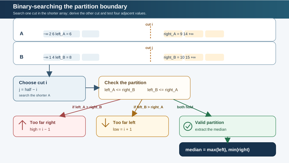
For a candidate pair (i, j), only four values matter:

left_A  = A[i - 1]   # greatest value on A's left
right_A = A[i]       # smallest value on A's right

left_B  = B[j - 1]   # greatest value on B's left
right_B = B[j]       # smallest value on B's right

If a side is empty, use a sentinel:

• Empty left side: negative infinity.
• Empty right side: positive infinity.

In Python:

left_A = float("-inf") if i == 0 else A[i - 1]
right_A = float("inf") if i == m else A[i]

left_B = float("-inf") if j == 0 else B[j - 1]
right_B = float("inf") if j == n else B[j]

The arrays are already sorted, so each array's own left side is ordered before its own right side. The only ordering that remains to verify is across the arrays:

left_A <= right_B
left_B <= right_A

These are the two nontrivial cross-boundary inequalities. Together, they certify that no value stranded on the left exceeds a value on the right.

The full local boundary picture is:

left_A  <= right_A
left_A  <= right_B

left_B  <= right_A
left_B  <= right_B

The first and fourth relationships are inherited from the sorted inputs. The middle two are the actual partition checks.

Duplicates are why these comparisons must be non-strict. If left_A == right_B, the cut is valid. Replacing <= with < rejects legitimate partitions.

Deriving the binary-search direction

Maintain the interval invariant:

Every still-possible valid partition index i lies in [low, high].

There are three cases.

Case 1: too many elements from A

If:

left_A > right_B

then an element from A's left side is too large to remain left of B's right side. The cut in A is too far right.

Move left:

high = i - 1

Every larger value of i would include at least as many elements from A on the left, so it cannot repair the ordering.

Case 2: too few elements from A

If:

left_B > right_A

then B contributes a value to the left that is larger than a value still on A's right side. The cut in A is too far left.

Move right:

low = i + 1

Taking more elements from A and therefore fewer from B is the only direction that can repair this crossing.

Case 3: valid partition

If both cross inequalities hold:

left_A <= right_B and left_B <= right_A

the partition is globally ordered. Stop searching.

This is binary search over a structural feasibility condition. We are not asking whether a number is present. We are asking whether a proposed cut can separate the combined sorted order.

Read the median from a valid partition

At a valid partition, the left side contains exactly:

left_size = (m + n + 1) // 2

elements.

The two cross inequalities imply that every value on the left is less than or equal to every value on the right. Therefore, the largest value on the left sits immediately before the right side:

left_max = max(left_A, left_B)

Likewise, the smallest value on the right is:

right_min = min(right_A, right_B)

The arithmetic now follows from the total length.

Odd total

When m + n is odd, the left side contains one extra element. Its largest value is the sole middle value:

median = left_max

Even total

When m + n is even, the two sides have equal size. The two central values are the largest value on the left and the smallest value on the right:

median = (left_max + right_min) / 2

The formulas are not a trick added after the search. They are forced by the partition invariant.

Worked trace

Take:

A = [1, 3]
B = [2, 4]

The total length is 4, so:

left_size = (4 + 1) // 2 = 2

Start with a candidate cut:

i = 1
j = left_size - i = 1

The partition is:

A: [1 | 3]
B: [2 | 4]

The boundaries are:

left_A  = 1
right_A = 3
left_B  = 2
right_B = 4

Check the cross inequalities:

left_A <= right_B   -> 1 <= 4
left_B <= right_A   -> 2 <= 3

The partition is valid.

Because the total is even:

left_max  = max(1, 2) = 2
right_min = min(3, 4) = 3

median = (2 + 3) / 2 = 2.5

We never merged the arrays. We only located the boundary around the two central values.

Implement the proof in Python

The implementation should mirror the derivation. Every variable has a job:

• A is the shorter array, so the search is logarithmic in the smaller input.
• left_size fixes the number of elements on the left.
• i is the searched partition.
• j is the complementary partition.
• The four boundary values determine feasibility.
• low and high preserve the remaining candidate interval.

from typing import List


def find_median_sorted_arrays(nums1: List[int], nums2: List[int]) -> float:
    # Search the shorter array.
    if len(nums1) > len(nums2):
        nums1, nums2 = nums2, nums1

    A, B = nums1, nums2
    m, n = len(A), len(B)
    total = m + n

    # The extra element goes on the left for odd totals.
    left_size = (total + 1) // 2

    low, high = 0, m

    while low <= high:
        i = (low + high) // 2
        j = left_size - i

        left_A = float("-inf") if i == 0 else A[i - 1]
        right_A = float("inf") if i == m else A[i]

        left_B = float("-inf") if j == 0 else B[j - 1]
        right_B = float("inf") if j == n else B[j]

        # The cut is globally valid.
        if left_A <= right_B and left_B <= right_A:
            left_max = max(left_A, left_B)

            if total % 2 == 1:
                return float(left_max)

            right_min = min(right_A, right_B)
            return (left_max + right_min) / 2.0

        # A contributes too many elements to the left.
        if left_A > right_B:
            high = i - 1
        else:
            # A contributes too few elements to the left.
            low = i + 1

    # Under the stated contract, sorted inputs guarantee a valid partition.
    raise ValueError("Inputs do not satisfy the sorted-array contract")

// is used for partition counts because i, j, and left_size must be integers. The final / is ordinary division because an even-length median may be fractional.

The sentinel values are implementation details that preserve one comparison model at the edges. Without them, every candidate cut needs separate branches for an empty left or right side. With them, i == 0 and i == m behave like ordinary cuts.

The defensive ValueError should be unreachable for valid sorted inputs. It is useful during debugging because it distinguishes a broken implementation or invalid precondition from a legitimate median result.

Common mistakes are predictable:

• Searching the longer array and allowing the complementary cut to fall outside B.
• Using strict < comparisons and rejecting duplicates.
• Forgetting that i may be 0 or len(A).
• Indexing A[i - 1], A[i], B[j - 1], or B[j] without guarding the boundaries.
• Returning max(left_A, left_B) for an even total instead of averaging both central values.
• Using ordinary division when calculating partition counts.
• Merging “temporarily” and accidentally violating the time requirement.

The short code is the final artifact. The invariant is the real solution.

Stress-test the boundaries, not just the example

A happy-path example proves very little here. The bugs live at empty sides, extreme cuts, parity changes, and equality.

Candidate cut too far right

Consider:

A = [4, 5]
B = [1, 2, 3, 6, 7]

The total is 7, so:

left_size = 4

Suppose:

i = 2
j = 2

The boundaries are:

left_A  = 5
right_A = +inf
left_B  = 2
right_B = 3

The inequality:

left_A <= right_B

fails because 5 > 3.

Too many elements were taken from A. The only valid direction is left:

high = i - 1

Candidate cut too far left

Consider:

A = [1, 2]
B = [3, 4, 5]

The total is 5, so:

left_size = 3

If:

i = 1
j = 2

the boundaries are:

left_A  = 1
right_A = 2
left_B  = 4
right_B = 5

Now:

left_B <= right_A

fails because 4 > 2.

A contributes too few elements to the left, so move right:

low = i + 1

The next cut can be:

i = 2
j = 1

which yields a valid partition and median 3.

Edge-case table

Case	What it tests	Boundary behavior
A = [], B = [2, 4, 5]	Empty input array	left_A or right_A becomes a sentinel
A = [1], B = []	Single combined element	Both cuts can be at an extreme
A = [1, 2], B = [3]	Odd total	left_max is the median
A = [1, 2], B = [3, 4]	Even total	Average left_max and right_min
A = [1, 2, 2], B = [2, 2]	Duplicates	<= must accept equal boundaries
A = [1, 2], B = [10, 11, 12]	Disjoint ranges	Valid cut may place all of A on the left
Inputs with reversed lengths	Normalization	Swap references before searching
Values near the allowed limits	Arithmetic boundaries	Sentinels remain outside real data

Some valid partitions occur at the beginning or end of the shorter array:

A = [1, 2]
B = [10, 11, 12, 13]

A valid cut can take all of A on the left. That is why high must start at len(A), not len(A) - 1.

The numeric constraints in the canonical problem keep real values well away from Python's infinity sentinels. More generally, the sentinel approach is safe when the sentinel values cannot collide with legitimate input values.

Correctness and complexity

The correctness argument has three parts.

First, left_size fixes the number of elements on the left. Since j = left_size - i, every candidate partition has the required total left-side size.

Second, the valid-partition conditions:

left_A <= right_B
left_B <= right_A

ensure that the largest value contributed by either left side does not exceed the smallest value contributed by the other right side. Combined with the sorted order inside each array, every left-side element is less than or equal to every right-side element.

Third, the median is therefore determined by the boundary values:

• Odd total: max(left_A, left_B).
• Even total: average of max(left_A, left_B) and min(right_A, right_B).

The binary-search interval remains valid because each failed inequality eliminates an entire direction:

• left_A > right_B eliminates the current and all larger i.
• left_B > right_A eliminates the current and all smaller i.

A valid partition exists because the two sorted arrays can be viewed as one sorted sequence with a cut after left_size elements. The search interval shrinks after every iteration, so it terminates.

Complexity:

Time:  O(log(min(m, n)))
Space: O(1)

The algorithm reads only a constant number of values per iteration. It does not merge, copy, sort, or allocate an output array.

For an interview, I would review the implementation in this order:

1. Did you swap so the binary search uses the shorter array?
2. Is left_size = (m + n + 1) // 2?
3. Is j derived as left_size - i?
4. Are all four boundaries guarded?
5. Are both cross inequalities checked with <=?
6. Does the direction match the violated inequality?
7. Are odd and even totals handled separately?
8. Have you tested empty sides, extreme cuts, duplicates, and both parities?

The transferable partition rule

The pattern signal is specific:

Two sorted regions must behave like one globally sorted sequence, but the answer depends only on a boundary near the middle.

That should suggest a partition binary search.

Do not search for the median value directly. Search for how many elements belong on the left from one sorted region. Derive the other count. Then compare the values immediately around the cut.

The reusable derivation is:

1. Write the required left-side size.
2. Choose one partition variable.
3. Derive the complementary partition.
4. Name the four boundary values.
5. Handle empty sides with sentinels.
6. Identify the violated cross-boundary inequality.
7. Move the cut in the only direction that can repair it.
8. Read the result from the boundaries once the cut is valid.

A logarithmic median algorithm is not a clever formula. It is a small proof made executable.

When two sorted regions need to become one ordered split, search the cut on the shorter region, let the complementary cut follow, and let the first violated boundary inequality choose the direction. Then test the places where the cut disappears: empty sides, beginning cuts, ending cuts, duplicates, odd totals, and even totals.

References

Research updated Sep 7, 2026