Set Matrix Zeroes

The dangerous part is not writing zeroes. It is remembering which zeroes were causes and which zeroes were created by your own writes.

The contract and the cascading trap

Given an m × n integer matrix, every row and column containing a zero in the original matrix must become entirely zero. The matrix must be modified in place.

That word—original—drives the whole solution.

Consider:

[
  [1, 1, 1],
  [1, 0, 1],
  [1, 1, 1]
]

The zero at (1, 1) means the final matrix should be:

[
  [1, 0, 1],
  [0, 0, 0],
  [1, 0, 1]
]

A tempting approach is to scan the matrix and immediately clear the row and column whenever you find a zero. But after clearing row 1, the cells (1, 0) and (1, 2) are new zeroes. If the scan later treats those cells as original triggers, it may clear additional rows and columns.

The transformation starts creating evidence that looks like input.

Core rule: discover all original zero-containing rows and columns first. Mutate the matrix only after discovery is complete.

The straightforward solution uses separate row and column tracking. The constant-space solution keeps the same two-phase logic, but stores the tracking information inside the matrix itself.

Build the baseline before compressing it

First make the required state explicit.

Create:

• zero_rows[i]: whether row i contained an original zero.
• zero_cols[j]: whether column j contained an original zero.

Then use two passes:

1. Scan every cell and record its row and column when the cell is zero.
2. Scan every cell again. Set it to zero if its row or column was recorded.

Conceptually:

for i in range(m):
    for j in range(n):
        if matrix[i][j] == 0:
            zero_rows[i] = True
            zero_cols[j] = True

for i in range(m):
    for j in range(n):
        if zero_rows[i] or zero_cols[j]:
            matrix[i][j] = 0

This version is useful even when the interview requires O(1) auxiliary space because it exposes the actual obligations:

• Every row marker answers, “Did this row originally contain a zero?”
• Every column marker answers, “Did this column originally contain a zero?”
• The second pass applies the recorded facts.

The baseline takes O(mn) time and O(m + n) auxiliary space.

The optimization is now precise: we do not need a different algorithm. We need a cheaper place to store the same row and column facts.

Reuse the matrix as marker storage

The matrix already contains convenient marker locations:

• matrix[i][0] can represent row i.
• matrix[0][j] can represent column j.

When an original zero appears at an interior position (i, j), write:

matrix[i][0] = 0
matrix[0][j] = 0

Those writes record the row and column obligations.

The first row and first column create the complication. Their cells are both ordinary input data and marker storage. In particular, the shared corner cannot independently represent these two facts:

• The first row originally contained a zero.
• The first column originally contained a zero.

One cell cannot carry two independent Boolean values. Preserve those facts in two scalar flags:

first_row_zero = False
first_col_zero = False

The storage layout is:

Storage	Responsibility
matrix[i][0] for i > 0	Row-marker information, possibly combined with an original first-column zero
matrix[0][j] for j > 0	Column-marker information, possibly combined with an original first-row zero
first_row_zero	Whether the original first row contained a zero
first_col_zero	Whether the original first column contained a zero

The word “possibly” matters. A zero in the first column can make matrix[i][0] zero even when row i has no interior zero. That is still safe: the entire row must be zeroed anyway because it already contained an original boundary zero. The same reasoning applies to a zero in the first row.

Partition the causes before writing the invariant

Every required zero in the final matrix comes from one of three sources:

1. An original zero at an interior position (i, j) where i > 0 and j > 0.
2. An original zero somewhere in the first row.
3. An original zero somewhere in the first column.

Store each cause through a dedicated path:

• Interior zeroes write a row marker and a column marker.
• First-row zeroes are summarized by first_row_zero.
• First-column zeroes are summarized by first_col_zero.

There can be overlap. For example, an original zero in the first column makes a row marker location zero. That does not corrupt the algorithm; it combines two facts that lead to the same consequence: the row must be cleared.

The traversal therefore has four stages:

1. Inspect the first row and save first_row_zero.
2. Inspect the first column and save first_col_zero.
3. Scan only the interior to write row and column markers.
4. Mutate the interior, then clean up the first row and first column.

Boundary cleanup must happen last because the boundary still contains working metadata.

Prove the two-phase invariant

Discovery invariant

After the discovery phase:

• If an interior zero was found in row i, then matrix[i][0] == 0.
• If an interior zero was found in column j, then matrix[0][j] == 0.
• If matrix[i][0] == 0, then either row i contains an interior zero or the original first-column cell (i, 0) was zero.
• If matrix[0][j] == 0, then either column j contains an interior zero or the original first-row cell (0, j) was zero.
• first_row_zero records whether the original first row contained a zero.
• first_col_zero records whether the original first column contained a zero.

This is deliberately weaker than claiming that every zero marker came only from an interior discovery. Boundary zeroes can also occupy marker locations. The weaker invariant is the correct one, and it is exactly strong enough for the mutation phase.

Mutation boundary

No interior cell is transformed until discovery is complete.

That prevents false cascades. A zero written during the mutation phase cannot be inspected as a new cause because the algorithm has already finished discovering causes.

The matrix is being used as storage, but storage and transformation remain separate phases. That separation matters more than the specific marker locations.

Interior mutation invariant

For every interior cell (i, j):

i > 0 and j > 0

the condition

matrix[i][0] == 0 or matrix[0][j] == 0

is true exactly when the final result requires (i, j) to become zero.

Why?

• If matrix[i][0] == 0, then either row i had an interior zero or its original first-column cell was zero. Both cases require the entire row to become zero.
• If matrix[0][j] == 0, then either column j had an interior zero or its original first-row cell was zero. Both cases require the entire column to become zero.
• If neither marker is zero, row i has no recorded interior or first-column cause, and column j has no recorded interior or first-row cause. No original zero requires this cell to change.

Therefore the update is both necessary and sufficient:

if matrix[i][0] == 0 or matrix[0][j] == 0:
    matrix[i][j] = 0

The two saved flags then handle the first row and first column independently.

Correctness has two halves: a zero marker proves that a cell must change; a nonzero marker proves that no recorded original cause requires it to change.

Dry-run a mixed boundary case

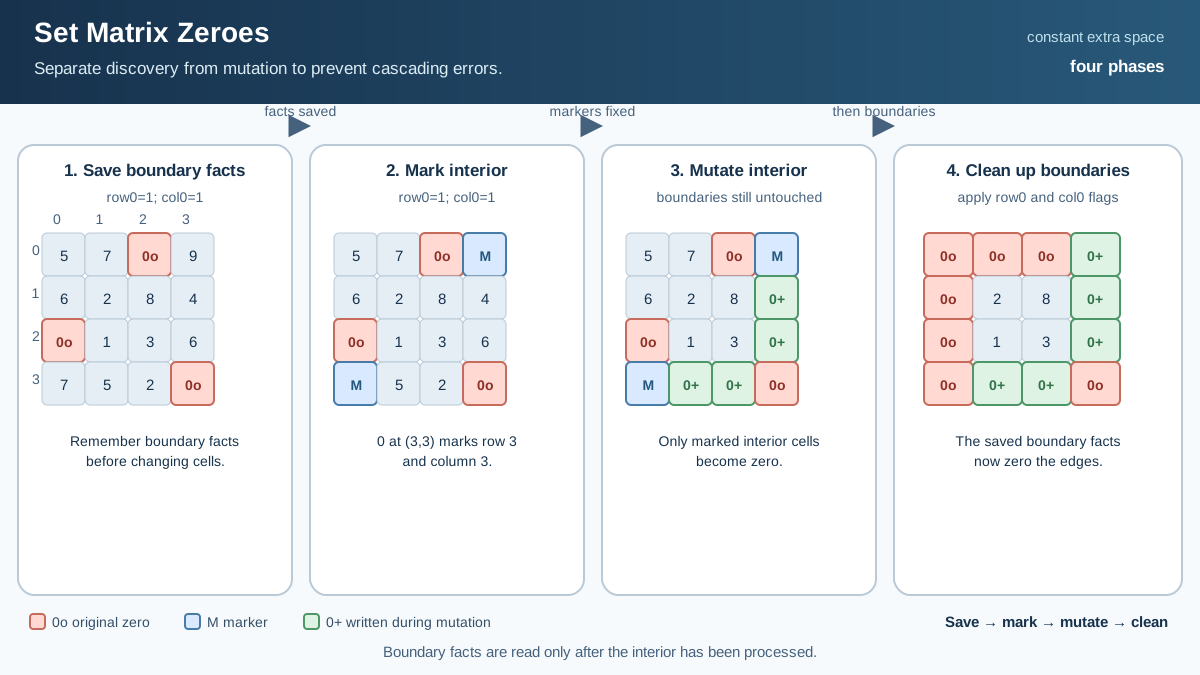
A boundary-only example checks the flags, but the delicate case combines boundary zeroes with an interior zero:

[
  [1, 2, 0, 4],
  [5, 6, 7, 8],
  [0, 10, 11, 12],
  [13, 14, 15, 0]
]

There is:

• A zero in the first row at (0, 2).
• A zero in the first column at (2, 0).
• An interior zero at (3, 3).

Step 1: Save boundary facts

The first row contains a zero:

first_row_zero = True

The first column also contains a zero:

first_col_zero = True

Step 2: Mark interior discoveries

The interior zero at (3, 3) writes:

matrix[3][0] = 0
matrix[0][3] = 0

After discovery, the relevant boundary state is:

[
  [1, 2, 0, 0],
  [5, 6, 7, 8],
  [0, 10, 11, 12],
  [0, 14, 15, 0]
]

The zero at matrix[2][0] comes from the original first-column zero. The zero at matrix[3][0] is an interior row marker. Both correctly imply that those rows must eventually be cleared.

The zero at matrix[0][2] comes from the original first-row zero. The zero at matrix[0][3] is an interior column marker. Both correctly imply that those columns must eventually be cleared.

Step 3: Mutate the interior

For the interior:

• Column 2 is marked, so interior cells in column 2 become zero.
• Column 3 is marked, so interior cells in column 3 become zero.
• Row 2 has a zero in its first-column marker location, so its interior cells become zero.
• Row 3 has an interior row marker, so its interior cells become zero.

After the interior pass:

[
  [1, 2, 0, 0],
  [5, 6, 0, 0],
  [0, 0, 0, 0],
  [0, 0, 0, 0]
]

Step 4: Clean up the boundaries

Because first_row_zero is true, clear the first row.

Because first_col_zero is true, clear the first column.

The final result is:

[
  [0, 0, 0, 0],
  [0, 6, 0, 0],
  [0, 0, 0, 0],
  [0, 0, 0, 0]
]

The zeroes created during the interior pass never become new discoveries. Discovery was already finished.

Implement the Python solution

class Solution:
    def setZeroes(self, matrix: list[list[int]]) -> None:
        # The problem contract uses a nonempty matrix.
        # This guard also keeps the function safe for general callers.
        if not matrix or not matrix[0]:
            return

        rows = len(matrix)
        cols = len(matrix[0])

        # Preserve the boundary facts that cannot be stored independently
        # in matrix[0][0].
        first_row_zero = any(matrix[0][j] == 0 for j in range(cols))
        first_col_zero = any(matrix[i][0] == 0 for i in range(rows))

        # Discovery phase:
        # The first column stores row information.
        # The first row stores column information.
        # Scan only the interior so marker writes are not rediscovered.
        for i in range(1, rows):
            for j in range(1, cols):
                if matrix[i][j] == 0:
                    matrix[i][0] = 0
                    matrix[0][j] = 0

        # Mutation phase for the interior.
        for i in range(1, rows):
            for j in range(1, cols):
                if matrix[i][0] == 0 or matrix[0][j] == 0:
                    matrix[i][j] = 0

        # Boundary cleanup happens after the markers are no longer needed.
        if first_row_zero:
            for j in range(cols):
                matrix[0][j] = 0

        if first_col_zero:
            for i in range(rows):
                matrix[i][0] = 0

Each state variable has one job:

• rows and cols define the traversal bounds.
• first_row_zero preserves the first-row obligation.
• first_col_zero preserves the first-column obligation.
• The first column stores row-related state.
• The first row stores column-related state.

The code is intentionally split into discovery, interior mutation, and boundary cleanup. Compressing the space should not compress the reasoning.

An implementation can use one boundary flag and infer the other from matrix[0][0], but two explicit flags are easier to derive and audit. The O(1) requirement concerns asymptotic auxiliary storage; it does not require eliminating every scalar variable.

Complexity and failure checks

The algorithm performs a constant number of scans:

• One scan of the first row.
• One scan of the first column.
• One interior discovery pass.
• One interior mutation pass.
• Up to two boundary cleanup passes.

Therefore:

Time:  O(mn)
Space: O(1) auxiliary space

The matrix itself is reused as marker storage. The additional memory consists only of scalar variables and loop state.

Check these cases before trusting the implementation:

• No zeroes: no markers are written, so the matrix remains unchanged.
• Zero at (0, 0): both boundary flags become true; both the first row and first column must be cleared.
• Zeroes only in the first row: clear the first row, but do not clear unrelated rows.
• Zeroes only in the first column: clear the first column, but do not clear unrelated columns.
• One row: the first-row flag handles the entire matrix; there is no interior row.
• One column: the first-column flag handles the entire matrix; there is no interior column.
• Multiple zeroes: repeatedly writing the same marker is harmless because zero is idempotent here.

The common failure modes are more useful than the happy path:

1. Mutating while discovering
   Generated zeroes are mistaken for original causes, producing a cascade.

2. Using matrix[0][0] for both boundary facts
   One cell cannot encode two independent conditions.

3. Treating marker values as exact historical evidence
   A marker location may be zero because of an interior zero or because the corresponding boundary cell was originally zero. The algorithm needs a sufficient condition for mutation, not a perfect reconstruction of history.

4. Clearing the marker row or column too early
   Those cells are working memory. Erase them only after the interior pass consumes them.

5. Returning a new matrix
   The contract requires modifying the supplied nested list in place. The method returns None.

My interview rule is simple: first derive the O(m + n)-space version. Name exactly what its arrays remember. Then ask whether the input has safe locations that can hold the same state.

Here, the first row and first column provide those locations. Their shared corner is the overlap, so preserve the two boundary facts with flags. Once you separate causes from consequences, the constant-space solution stops looking like a memorized trick.

When output depends on properties of the original input, separate observation from mutation. If extra storage is expensive, reuse safe regions of the input as metadata—but preserve any information lost when those regions overlap.

First record the causes. Then apply the consequences. That is the reasoning move to carry into the next in-place marking problem.

References

Research updated Sep 7, 2026