Minimum Path Sum

Stop tracing paths. Track the cheapest cost that reaches each cell.

The right Minimum Path Sum solution is a two-dimensional dynamic program. For every coordinate, store the minimum sum needed to reach it from the top-left. Because movement is restricted to right and down, each cell has at most two legal predecessors: the cell above and the cell to the left.

That gives us an O(mn) algorithm instead of repeatedly exploring the same paths.

Read the Problem Contract

The input is an m x n grid of non-negative numbers.

Starting at grid[0][0], you may move only:

• Down: (i, j) -> (i + 1, j)
• Right: (i, j) -> (i, j + 1)

Return the minimum sum of cell values along a path to grid[m - 1][n - 1].

The values of both endpoints count. The task asks for the sum, not the path itself.

The dimensions satisfy 1 <= m, n <= 200, so the grid contains at most 40,000 cells. Enumerating every possible route is the wrong scale: the number of right/down paths grows combinatorially, and recursive exploration revisits the same intermediate coordinates many times.

The reusable object is smaller than a complete path:

What is the cheapest way to reach this coordinate?

That question leads directly to dynamic programming.

Recognize the Two-Predecessor Pattern

A brute-force recursive solution would stand at each cell and branch:

1. Try moving down.
2. Try moving right.
3. Keep the cheaper completed route.

This produces the right conceptual recurrence, but without memoization it recomputes subproblems. For example, several different prefixes can eventually ask for the best route through the same cell. The recursion keeps rediscovering an answer that should have been stored once.

Define the state:

dp[i][j] = minimum path sum from (0, 0) to (i, j)

The row and column coordinates are meaningful state dimensions. Moving to a different row or column changes the set of legal prefixes that can reach the cell, so one scalar value cannot represent the entire problem.

Now inspect the geometry. A path can enter (i, j) only from:

• Above: (i - 1, j)
• Left: (i, j - 1)

There are no other legal predecessors. That fixed predecessor set is the recognition cue for this 2D dynamic programming grid.

We fill the table row by row. When computing (i, j), both its top and left states have already been computed.

Derive the Recurrence and Borders

For an interior cell, choose the cheaper predecessor and add the current cell's value:

dp[i][j] = grid[i][j] + min(dp[i - 1][j], dp[i][j - 1])

Why is it enough to keep only the cheaper route to each predecessor?

Suppose the final move into (i, j) comes from above. Any route using that move shares the same suffix: grid[i][j]. If one route to (i - 1, j) is already more expensive than another, extending both routes with the same current value cannot make the expensive prefix win.

This is the optimal-substructure property:

An optimal path to a cell contains an optimal path to the predecessor it uses.

The borders need separate treatment because they have only one possible predecessor.

Start cell

The starting cell has no predecessor:

dp[0][0] = grid[0][0]

First row

Every cell in the first row can only be reached from the left:

dp[0][j] = dp[0][j - 1] + grid[0][j]

These are cumulative sums across the row.

First column

Every cell in the first column can only be reached from above:

dp[i][0] = dp[i - 1][0] + grid[i][0]

These are cumulative sums down the column.

A common mistake is to treat a missing predecessor as 0. That invents a cheap route through an edge. For example, if you compute the first interior cell using min(top, left) while one nonexistent predecessor is zero, the algorithm may pretend the path entered the grid from outside.

You can avoid explicit border loops with an infinity sentinel, but the underlying rule does not change: an unavailable predecessor must never compete as a valid zero-cost route.

Prove the State Invariant

The implementation is correct if this invariant remains true:

After dp[i][j] is computed, it equals the minimum cost of every legal path from (0, 0) to (i, j).

The proof follows row-major order.

• At (0, 0), the only path consists of the starting cell, so the initialization is correct.
• Along the first row, there is only one possible direction: right. The cumulative initialization therefore gives the only possible path cost.
• Along the first column, there is only one possible direction: down. The cumulative initialization is again forced.
• For an interior cell, every legal path must arrive from above or from the left. By the invariant, dp[i - 1][j] and dp[i][j - 1] already contain the cheapest costs to those predecessors. Choosing the smaller one and adding grid[i][j] gives the cheapest route to the current cell.

Therefore dp[m - 1][n - 1] is the minimum path sum for the entire grid.

For debugging, inspect any interior cell and check:

stored value == grid value + min(already-computed top, already-computed left)

That small local check catches incorrect loop order, wrong indices, and accidental use of the original grid instead of the DP table.

Dry-Run the DP Table

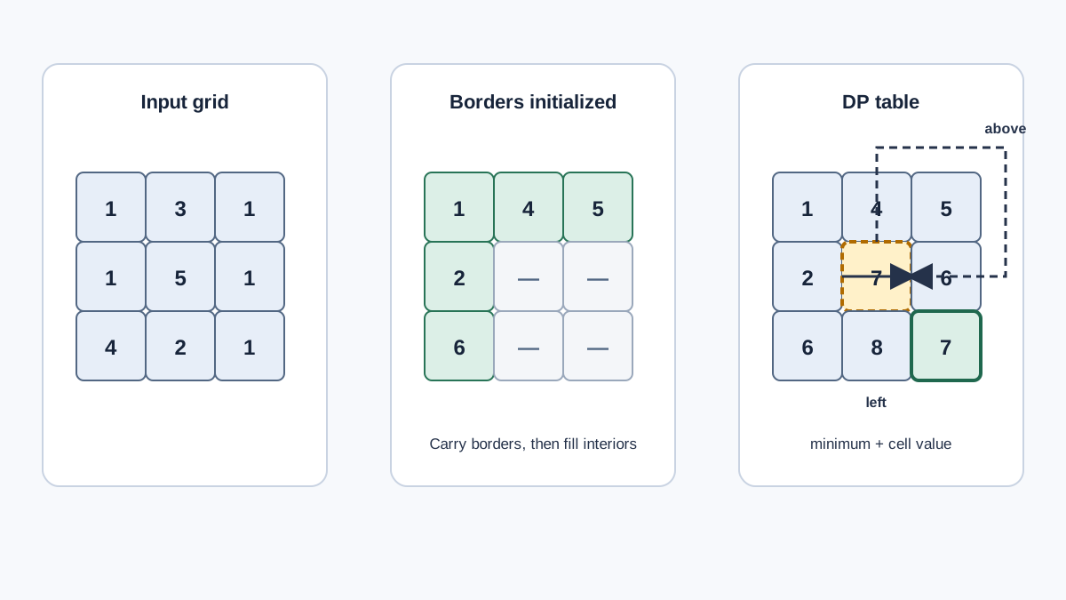
Use this grid:

1  3  1
1  5  1
4  2  1

Start with the top-left cell:

1  0  0
0  0  0
0  0  0

Fill the first row using cumulative sums:

• dp[0][1] = 1 + 3 = 4
• dp[0][2] = 4 + 1 = 5

Fill the first column:

• dp[1][0] = 1 + 1 = 2
• dp[2][0] = 2 + 4 = 6

The table now looks like this:

1  4  5
2  0  0
6  0  0

Now compute the interior cells.

At (1, 1):

dp[1][1] = 5 + min(dp[0][1], dp[1][0])
         = 5 + min(4, 2)
         = 7

At (1, 2):

dp[1][2] = 1 + min(5, 7) = 6

At (2, 1):

dp[2][1] = 2 + min(7, 6) = 8

At (2, 2):

dp[2][2] = 1 + min(6, 8) = 7

The completed table is:

1  4  5
2  7  6
6  8  7

The answer is 7.

One corresponding minimum-cost route is:

1 -> 3 -> 1 -> 1 -> 1

The table records costs, not route choices. That is enough for this problem. Reconstructing the route would require storing predecessor choices or walking backward through the completed table, but neither is necessary when only the sum is requested.

Single-cell, single-row, and single-column grids are useful checks:

• A single cell returns its own value.
• A single row returns the sum of that row.
• A single column returns the sum of that column.

Implement the 2D Solution in Python

I prefer a fresh DP table for the primary implementation. It keeps the original input unchanged and makes every subproblem visible while debugging.

def min_path_sum(grid: list[list[int]]) -> int:
    rows, cols = len(grid), len(grid[0])

    # dp[i][j] is the minimum cost to reach (i, j).
    dp = [[0] * cols for _ in range(rows)]

    dp[0][0] = grid[0][0]

    # The first column can only be reached from above.
    for i in range(1, rows):
        dp[i][0] = dp[i - 1][0] + grid[i][0]

    # The first row can only be reached from the left.
    for j in range(1, cols):
        dp[0][j] = dp[0][j - 1] + grid[0][j]

    # Every interior cell has top and left predecessors.
    for i in range(1, rows):
        for j in range(1, cols):
            dp[i][j] = grid[i][j] + min(
                dp[i - 1][j],
                dp[i][j - 1],
            )

    return dp[rows - 1][cols - 1]

There are three visible decisions in this code:

1. The state meaning is explicit.
2. The borders are initialized according to their actual geometry.
3. The destination state is returned because it represents the cheapest cost to reach the target.

You could mutate grid directly and use it as the DP table. That reduces allocation, but it changes caller-owned data. Unless the problem explicitly permits mutation, the separate table is the safer interview choice.

Compress the Table to One Row

The full table stores more history than the recurrence needs.

When computing (i, j), we need only:

• The value above: the previous row's dp[j]
• The value to the left: the current row's already-updated dp[j - 1]

That means one array is enough.

Use this invariant:

After processing a row through column j, dp[j] is the minimum cost to reach the cell at column j in the current row.

The update must move left to right:

dp[j] = grid[i][j] + min(dp[j], dp[j - 1])

Before the assignment:

• dp[j] represents the cell above.
• dp[j - 1] represents the cell to the left.

After the assignment, dp[j] represents the current cell.

def min_path_sum_optimized(grid: list[list[int]]) -> int:
    rows, cols = len(grid), len(grid[0])

    # dp[j] initially represents the best cost to the cell
    # in the first row at column j.
    dp = [float("inf")] * cols
    dp[0] = 0

    for i in range(rows):
        # dp[j] is "above"; dp[j - 1] is "left".
        for j in range(cols):
            dp[j] = grid[i][j] + min(dp[j], dp[j - 1])

    return dp[-1]

The sentinel initialization handles the borders without separate loops:

• At (0, 0), dp[0] starts at 0, so the first update becomes grid[0][0].
• At the first column of later rows, dp[j - 1] is the valid left boundary state and dp[j] remains infinity, so the update must come from above.
• At the first row, the previous-row values are infinity except for the start, so the updates propagate from left to right.

The traversal direction is part of the algorithm. If you process columns right to left, dp[j - 1] no longer represents the current row's left neighbor. You have destroyed the dependency that the recurrence relies on.

The compressed version is cheaper in memory, but the tradeoff is real: once a value is overwritten, the full table is unavailable for inspection or straightforward route reconstruction.

Complexity and Failure Modes

For both implementations, every grid cell is processed once.

• Time: O(mn)
• Full-table auxiliary space: O(mn)
• One-row auxiliary space: O(n)

Here, n is the number of columns. If you want to minimize memory further, you can transpose the conceptual processing direction so the shorter dimension becomes the stored row, but the ordinary one-row implementation is usually clearer in an interview.

Check these cases before you trust the code:

• One cell
• One row
• One column
• Cells containing zero
• A target whose value must be included
• A start value that must be included
• The maximum 200 x 200 dimensions

The common failure modes are predictable:

• Using max instead of min
• Omitting grid[0][0]
• Omitting the destination value
• Using len(grid) for both dimensions
• Reading an uninitialized top or left predecessor
• Treating an unavailable predecessor as zero
• Updating the compressed array in the wrong direction
• Mutating the input without acknowledging the tradeoff

The non-negative, right/down contract gives this problem an acyclic dependency structure. Every move increases the row or column index, so the computation has a natural forward order.

The Interview Rule

When movement is one-way and each coordinate has a small fixed set of predecessors, stop thinking about complete paths. Define the best cost to reach each coordinate.

Then:

1. Name the state: dp[i][j].
2. List the legal predecessors.
3. Write the recurrence.
4. Initialize borders where predecessors are missing.
5. Choose an iteration order that computes dependencies first.
6. Compress space only after the full state dependency is clear.

Before writing code, say this sentence out loud:

dp[i][j] is the minimum cost to reach (i, j), and it depends on the best costs from above and from the left.

That sentence is the solution direction. The code is just the table filling.

References

Research updated Sep 7, 2026