Unique Paths

The reliable way to solve Unique Paths is to count paths to each cell, not to enumerate complete routes. Every cell has at most two meaningful predecessors: the cell above and the cell to its left.

Recognize the Path-Counting Structure

The problem gives an m x n grid. A robot starts at (0, 0), must reach (m - 1, n - 1), and may move only:

• Down: increase the row
• Right: increase the column

There are no obstacles or cell costs in this version. Every legal route contributes exactly one to the answer.

The key signals are:

1. We are counting ways.
2. Movement is monotone: rows and columns never decrease.
3. A cell is identified by two coordinates.
4. The ways to reach a cell depend on earlier cells.

That points directly to two-dimensional dynamic programming.

Define dp[r][c] as the number of valid paths from the start to cell (r, c). The answer is dp[m - 1][n - 1].

This state definition is the center of the solution. Once it is correct, the recurrence and traversal order follow from the grid's geometry.

Build the Brute-Force Recurrence

Start with the recursive question:

paths(r, c) = number of paths from (0, 0) to (r, c)

For an interior cell (r, c), the final move must come from one of two places:

• From above, (r - 1, c), by moving down
• From the left, (r, c - 1), by moving right

So:

paths(r, c) = paths(r - 1, c) + paths(r, c - 1)

The base and boundary rules are:

paths(0, 0) = 1
paths(r, c) = 0 if r < 0 or c < 0

The start cell has one path: the path that has taken no moves yet. A nonexistent predecessor contributes zero paths.

A recursive implementation could compute the destination by repeatedly asking for the cell above and the cell to the left. The problem is repeated work. To see it, consider the calls needed for a small interior cell:

paths(r, c)
├── paths(r - 1, c)
│   ├── paths(r - 2, c)
│   └── paths(r - 1, c - 1)
└── paths(r, c - 1)
    ├── paths(r - 1, c - 1)
    └── paths(r, c - 2)

The subproblem paths(r - 1, c - 1) appears in both branches. Larger grids create more overlap. The recursion tree keeps rediscovering the same coordinates.

That repeated coordinate is the leverage point. Cache one result per (r, c), or build those results iteratively in a table. The bottom-up table is easier to inspect in an interview because its state meaning remains visible.

Derive the 2D DP Table

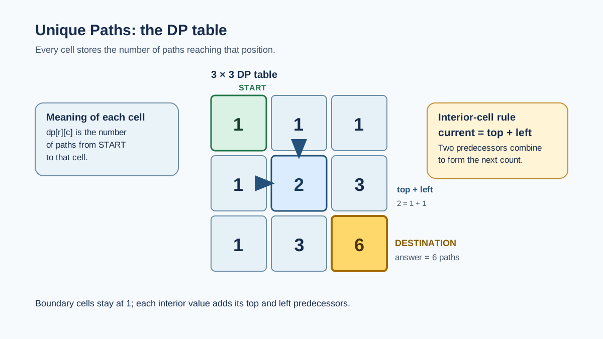
Let:

dp[r][c] = number of valid paths from (0, 0) to (r, c)

For every cell other than the start:

dp[r][c] = dp[r - 1][c] + dp[r][c - 1]

Why addition? Partition the paths by their final move. A path entering (r, c) either arrives from above or from the left. Those two groups contain all valid paths and do not overlap.

Boundary initialization

The first row can only be reached by moving right repeatedly. Therefore, every cell in row 0 has one path.

Likewise, the first column can only be reached by moving down repeatedly. Every cell in column 0 also has one path.

For example, a 3 x 3 table becomes:

1 1 1
1 2 3
1 3 6

The destination contains 6.

You can initialize the borders explicitly, or initialize only dp[0][0] = 1 and let the transition treat missing predecessors as zero. I prefer the second form in the first implementation because it keeps one recurrence for every non-start cell.

The traversal order must respect dependencies. In row-major order:

• dp[r - 1][c] has already been computed in the previous row.
• dp[r][c - 1] has already been computed earlier in the current row.

The table is a dependency map. Fill it in the direction the information flows.

Prove the Count Is Correct

The proof is short because the state matches the structure of the problem.

For a non-start cell (r, c), divide all valid paths to that cell into two groups:

1. Paths whose final move comes from (r - 1, c)
2. Paths whose final move comes from (r, c - 1)

This partition is:

• Complete: every legal path entering the cell must use either down from above or right from the left.
• Disjoint: a path has exactly one final move, so it cannot belong to both groups.

The first row and first column are correct because each has only one possible route from the start. The start itself has one path.

Now process cells in row-major order. Assume the states above and left of the current cell already contain their correct counts. By the partition argument, adding them gives exactly the number of paths to the current cell. That preserves the invariant for the next state.

By induction, every table entry is correct, including the destination.

DP invariant: when (r, c) is processed, dp[r][c] equals the number of valid paths from the start to that cell.

This invariant also gives you a debugging method. If a result is wrong, inspect the first cell where the invariant fails. Common causes are incorrect border handling, swapped dimensions, or reading a predecessor before it has been computed.

Implement the Python Solution

Start with the full table. It mirrors the proof directly.

class Solution:
    def uniquePaths(self, m: int, n: int) -> int:
        dp = [[0] * n for _ in range(m)]
        dp[0][0] = 1

        for r in range(m):
            for c in range(n):
                if r == 0 and c == 0:
                    continue

                if r > 0:
                    dp[r][c] += dp[r - 1][c]

                if c > 0:
                    dp[r][c] += dp[r][c - 1]

        return dp[m - 1][n - 1]

Each line has a direct obligation:

• dp[r][c] stores paths reaching one specific cell.
• The top predecessor is added only when it exists.
• The left predecessor is added only when it exists.
• The destination entry is the requested count.

There are no special cases for a one-row grid, a one-column grid, or a 1 x 1 grid:

• In a one-row grid, each cell accumulates only from the left.
• In a one-column grid, each cell accumulates only from above.
• In a 1 x 1 grid, the start is already the destination, so the answer is 1.

Compress the table to one row

The full table is the clearest version, but each cell needs only two values:

• The value above it from the previous row
• The value to its left in the current row

That allows a one-dimensional array:

class Solution:
    def uniquePaths(self, m: int, n: int) -> int:
        dp = [1] * n

        for r in range(1, m):
            for c in range(1, n):
                dp[c] += dp[c - 1]

        return dp[n - 1]

Here, dp[c] has two meanings during an update:

• Before the update, it is the value from above—the previous row.
• After the update, it is the value for the current row.

dp[c - 1] is already the current row's left value. Therefore:

new dp[c] = old dp[c] + current dp[c - 1]

The update direction matters. Process columns from left to right so dp[c - 1] represents the current row. If you process from right to left, you would read the old previous-row value for the left neighbor instead, breaking the dependency model.

I would explain the two-dimensional version first in an interview. It exposes the state and proof. If the interviewer asks for less memory, compress it afterward and state exactly what each array slot means.

Compare DP With Combinatorics

Dynamic programming counts paths cell by cell. There is also a direct mathematical view.

To reach the destination, every complete path must contain:

• m - 1 down moves
• n - 1 right moves

So each path has:

m + n - 2

total moves.

A path is therefore an arrangement of those moves. Choose which positions contain the down moves:

C(m + n - 2, m - 1)

Equivalently, choose the positions of the right moves:

C(m + n - 2, n - 1)

For a 3 x 2 grid, the robot needs two down moves and one right move. There are three arrangements:

D D R
D R D
R D D

So the answer is C(3, 2) = 3.

A carefully implemented multiplicative calculation can use O(1) auxiliary space and perform work proportional to the smaller number of move types. It should avoid computing factorials directly, which creates unnecessary intermediate arithmetic and implementation risk.

The combinatorial solution is elegant for this exact problem. But DP is the stronger interview pattern because it exposes the dependency structure. Change the problem so that some cells are blocked or movement rules depend on cell state, and the direct binomial formula no longer applies unchanged. The DP state can usually be extended by changing the transition.

That is the distinction worth remembering:

• Combinatorics counts complete move sequences directly.
• DP counts partial results and composes them through predecessor states.

Check Complexity and Edge Cases

For the full two-dimensional table:

• Time: O(mn), because every cell is processed once.
• Auxiliary space: O(mn), for the table.

For the one-dimensional version:

• Time: O(mn).
• Auxiliary space: O(n).

If you normalize the dimensions so the smaller dimension is used for the array, the compressed space can be O(min(m, n)).

Use these checks before submitting:

Case	Expected reasoning
m = 1	Only right moves are possible, so there is one path.
n = 1	Only down moves are possible, so there is one path.
m = n = 1	Start and destination are the same cell, so the answer is 1.
m = 3, n = 2	Two down moves and one right move produce 3 paths.

The most common failures are small and predictable:

• Counting m down moves instead of m - 1
• Counting n right moves instead of n - 1
• Initializing the start cell to 0
• Mixing up rows and columns
• Reading dp[r - 1][c] or dp[r][c - 1] without checking that it exists
• Updating a compressed array in the wrong direction
• Adding obstacle logic to this problem even though no obstacles are part of its contract

The last mistake matters in interviews. Neighboring grid problems may change the transition, but you should not silently solve a different problem. First implement the stated right/down path count. Extend the state only when the question adds a new constraint.

When a problem asks for the number of ways through a grid with monotone movement, inspect the final decision at each cell. If every state can be reached from a small set of already-computed predecessors, define the count-to-state, initialize the boundaries, and process the dependency graph in order.

Do not memorize the table. Derive it:

1. Name what one state counts.
2. Partition paths by the final move.
3. Initialize the start and boundaries.
4. Fill states only after their predecessors exist.
5. Return the destination state.

That is the reusable Unique Paths solution—and the real pattern is larger than this grid: count partial progress, preserve the invariant, and let the dependency structure dictate the code.

References

Research updated Sep 7, 2026