Unique Paths II

The recurrence is familiar. The interview usually turns on the cells you forgot: a blocked start, a blocked destination, or an obstacle that permanently cuts a border.

The core rule is simple:

An open cell inherits paths from above and left. An obstacle contributes zero, so invalid paths stop propagating.

That gives an O(mn) dynamic programming solution. The important work is making the state meaning, initialization, and update order precise enough that the rule survives every edge case.

Recognize the path-counting structure

The grid contains open cells marked 0 and obstacles marked 1. The robot starts at (0, 0), must reach (m - 1, n - 1), and may move only right or down.

This is a path-counting problem with invalid states.

For any cell (r, c), the final move into that cell can come only from:

• Above: (r - 1, c)
• Left: (r, c - 1)

There are no other legal predecessor cells. Therefore, if the current cell is open, its path count is the sum of those two predecessor counts.

A brute-force recursive solution exposes the same structure:

paths(r, c) =
    paths(r - 1, c) + paths(r, c - 1)

But the recursion reaches the same cells through many different routes. For example, a cell near the middle of the grid may be needed by both a path that first moves down and a path that first moves right. Recomputing that subproblem creates an unnecessary branching tree.

Dynamic programming stores the result for each cell once. With at most 100 x 100 cells, straightforward tabulation is more than sufficient. We do not need a clever combinatorial formula; the obstacle pattern is local, and the grid is small enough to inspect cell by cell.

The distinction matters:

• Minimum Path Sum stores the cheapest cost to reach a cell.
• Unique Paths II stores the number of valid ways to reach a cell.

The grid shape is similar, but the state meaning and recurrence are different.

Define the state and answer early

Use a table with the same dimensions as the input:

dp[r][c] = number of valid paths from (0, 0) to (r, c)

The answer is therefore:

dp[m - 1][n - 1]

Now derive the transitions.

Open cell

If (r, c) is open, every valid path ending there must make its final move from above or from the left:

dp[r][c] = paths from above + paths from left

In code, missing neighbors contribute zero:

from_above = dp[r - 1][c] if r > 0 else 0
from_left = dp[r][c - 1] if c > 0 else 0

dp[r][c] = from_above + from_left

Obstacle

If obstacleGrid[r][c] == 1, no valid path may enter that cell:

dp[r][c] = 0

This zero does more than describe the obstacle itself. It cuts propagation. A later cell may read the zero from above or left, but it cannot accidentally count a route through the blocked cell.

Start cell

An open start has one path to itself: the path that has taken zero moves so far.

dp[0][0] = 1

If the start is blocked, no path exists at all:

if obstacleGrid[0][0] == 1:
    return 0

This is the first edge case to settle because every later state depends, directly or indirectly, on the start.

State invariant: Every computed dp[r][c] is the number of valid paths that reach (r, c) without entering an obstacle.

Once that sentence is true, the recurrence is no longer a memorized formula. It is a direct consequence of the problem.

Get borders and endpoints right

The first row and first column expose weak initialization.

On the first row, the robot can only move right. So the cells are reachable until the first obstacle. Once an obstacle appears, every cell to its right must remain unreachable.

For example:

obstacle grid:
0  0  1  0  0

path counts:
1  1  0  0  0

The open cell after the obstacle does not recover. There is no way to approach it from below because the first row has no cells above the grid.

The same logic applies to the first column:

obstacle grid:
0
0
1
0

path counts:
1
1
0
0

A common mistake is to initialize every first-row and first-column cell to 1. That works only when those borders contain no obstacles. The obstacle version requires a permanent cutoff.

The safest implementation is to avoid special border initialization altogether:

1. Create a table filled with zeroes.
2. Set the open start to 1.
3. Traverse in row-major order.
4. Read the top and left neighbors only when they exist.

Then the borders naturally use zero for missing neighbors, and an obstacle naturally leaves a zero behind.

Blocked destination

If the destination is blocked, it must remain zero. It does not matter that neighboring cells may have valid paths reaching the destination's coordinates. A path cannot enter an obstacle.

The normal traversal handles this if the obstacle check happens before the addition:

if obstacleGrid[r][c] == 1:
    dp[r][c] = 0
else:
    dp[r][c] = ...

If you add the neighbors first and check the obstacle afterward—or forget the check entirely—you count paths that end on an invalid cell.

A one-cell grid

A 1 x 1 grid is a useful sanity check:

• [[0]] has one path: stay at the start, which is also the destination.
• [[1]] has zero paths because the only cell is blocked.

The explicit start check handles both cases cleanly.

Prove the recurrence with row-major order

The implementation processes cells from top to bottom and left to right. Before processing (r, c):

• (r - 1, c) has already been processed if it exists.
• (r, c - 1) has already been processed if it exists.

That gives the dependency order required by the recurrence.

Now prove the invariant by induction over this traversal order.

Base case

For (0, 0):

• If it is blocked, the algorithm returns 0.
• If it is open, dp[0][0] = 1, representing the single zero-move path to the starting cell.

So the invariant holds at the start.

Obstacle case

Suppose (r, c) is an obstacle. No valid path can enter it, so the correct count is zero. The algorithm stores:

dp[r][c] = 0

Any later cell that depends on this cell receives zero from that direction. Therefore, paths cannot cross the obstacle through the table.

Open-cell case

Suppose (r, c) is open. Every valid path ending at (r, c) has exactly one final move:

• From above, or
• From the left.

These two groups are exhaustive: movement is limited to down and right.

They are also disjoint. A path cannot have both an above final move and a left final move. Therefore, adding the two predecessor counts counts every valid path exactly once:

dp[r][c] = dp[r - 1][c] + dp[r][c - 1]

The predecessor values are already correct because of row-major traversal. By induction, every table entry is correct, including the destination.

Correctness condition: The recurrence works because paths are partitioned by their final move, while obstacles are represented by zero states that cannot contribute to later cells.

Dry-run obstacles and dead ends

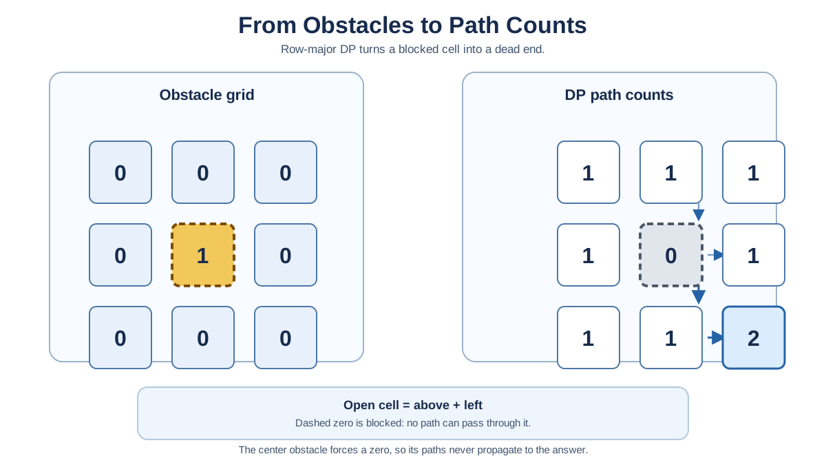
Consider this obstacle grid:

0  0  0
0  1  0
0  0  0

Fill the path-count table row by row:

1  1  1
1  0  1
1  1  2

At the center obstacle, the count is forced to zero. The cells around it still receive paths through the open border routes. The destination has two paths:

1. Right, right, down, down
2. Down, down, right, right

Now put the obstacle in the first row:

0  1  0
0  0  0

The table becomes:

1  0  0
1  1  1

The top-right cell is open, but it is unreachable. Its top neighbor is outside the grid, and its left neighbor is blocked. The zero keeps moving through the dead region.

For a blocked start:

1  0
0  0

The answer is immediately 0. There is no valid initial position from which to begin.

For a blocked destination:

0  0
0  1

The destination remains zero even though the cell above and the cell to the left are reachable:

1  1
1  0

This is the practical debugging test: inspect the table, not just the final number. A blocked cell should look like a zero valve. It stops incoming flow and prevents downstream counts from using that route.

Implement the clear Python tabulation

I would write the two-dimensional version first in an interview. It makes the state visible, keeps obstacle information separate from path counts, and gives you a table you can inspect while debugging.

from typing import List


class Solution:
    def uniquePathsWithObstacles(
        self, obstacleGrid: List[List[int]]
    ) -> int:
        rows = len(obstacleGrid)
        cols = len(obstacleGrid[0])

        if obstacleGrid[0][0] == 1:
            return 0

        dp = [[0] * cols for _ in range(rows)]
        dp[0][0] = 1

        for r in range(rows):
            for c in range(cols):
                if r == 0 and c == 0:
                    continue

                if obstacleGrid[r][c] == 1:
                    dp[r][c] = 0
                    continue

                if r > 0:
                    dp[r][c] += dp[r - 1][c]

                if c > 0:
                    dp[r][c] += dp[r][c - 1]

        return dp[rows - 1][cols - 1]

Each part answers a specific obligation:

• dp stores the number of valid paths to each cell.
• dp[0][0] = 1 establishes the zero-move base case.
• The obstacle branch prevents invalid cells from receiving or forwarding paths.
• The r > 0 and c > 0 guards make missing border neighbors contribute zero.
• Row-major traversal ensures both predecessors are ready before a cell is computed.

You could mutate the input grid and use it as the DP table, but that mixes two different meanings in one array: obstacle markers at first, path counts later. It saves memory, but it makes the state less obvious and can break callers that expect the input to remain unchanged. I prefer the separate table unless mutation is explicitly allowed and the space tradeoff matters.

Compress the table to one row

The 2D table stores more history than the recurrence needs.

When processing (r, c), the algorithm reads only:

• The value above: dp[r][c] before it is updated for the current row.
• The value to the left: dp[r][c - 1] after it has already been updated for the current row.

That lets one array represent both directions of dependency.

Use:

dp[c] = value from above
dp[c - 1] = value from the left

Scan each row from left to right:

from typing import List


class Solution:
    def uniquePathsWithObstacles(
        self, obstacleGrid: List[List[int]]
    ) -> int:
        rows = len(obstacleGrid)
        cols = len(obstacleGrid[0])

        if obstacleGrid[0][0] == 1:
            return 0

        dp = [0] * cols
        dp[0] = 1

        for r in range(rows):
            for c in range(cols):
                if obstacleGrid[r][c] == 1:
                    dp[c] = 0
                elif c > 0:
                    dp[c] += dp[c - 1]

        return dp[-1]

Consider an open cell. Before updating dp[c], it still contains the path count from the previous row—the value from above. dp[c - 1] already contains the current row's value from the left. Adding them applies the original recurrence without a second dimension.

For an obstacle, assign zero:

dp[c] = 0

That clears the old value from above. Without this assignment, paths from the previous row would leak through the obstacle.

The update order is part of the algorithm, not a style preference. Scanning right to left would destroy the meaning of dp[c - 1], and overwriting dp[c] before using it would destroy the above value. Compression works only because the array has a carefully maintained state interpretation.

Compressed-state invariant: During a left-to-right scan, dp[c] is the previous row's count until the current cell updates it, while dp[c - 1] is already the current row's count.

The compressed version uses the same recurrence as the 2D version. It simply keeps less history.

Verify complexity and reuse the rule

For both implementations, every grid cell is processed once and each update performs constant work.

Implementation	Time	Auxiliary space
2D tabulation	O(mn)	O(mn)
One-row tabulation	O(mn)	O(n)

Here, n is the number of columns. The one-row version is preferable when memory matters, but the 2D version is easier to explain and debug. In an interview, derive the clear version first. Compress only after you can name exactly what every read means.

Before submitting, test these cases:

• Blocked start
• Blocked destination
• 1 x 1 open grid
• 1 x 1 blocked grid
• One-row grid
• One-column grid
• Obstacle in the first row
• Obstacle in the first column
• Interior obstacle
• No possible route
• Multiple routes around an obstacle

The recurring bugs are narrow and predictable:

1. Counting through an obstacle.
2. Initializing every border cell to 1, even after a blockage.
3. Updating a compressed array in the wrong direction.
4. Confusing the obstacle grid with the DP state after mutating it.

The transferable rule is this:

When a grid state depends on a fixed set of already-solved neighbors, follow the dependency geometry. For path counting, make invalid cells zero so they cannot propagate; verify endpoint and border behavior; compress memory only after the state invariant is explicit.

Derive the 2D table on paper. Mark what each update reads. Then remove dimensions one at a time. That is how a compact solution stays correct instead of becoming a clever bug.

References

Research updated Sep 7, 2026